I was generated data of Ads Data, Leads Data, and Sales Data as below
this is the Ads Data result of the generated
| campaign_id | source | date | impressions | clicks | spend | leads | cpl | conversions |
|---|---|---|---|---|---|---|---|---|
| Google_Camp1 | 2024-01-01 | 8270 | 485 | 955.64 | 485 | 1.97 | 310 | |
| Google_Camp2 | 2024-01-01 | 6501 | 185 | 496.54 | 185 | 2.68 | 118 | |
| Google_Camp3 | 2024-01-01 | 3902 | 301 | 272.83 | 301 | 0.91 | 192 | |
| TikTok_Camp1 | TikTok | 2024-01-01 | 3339 | 310 | 984.18 | 310 | 3.17 | 198 |
| TikTok_Camp2 | TikTok | 2024-01-01 | 6729 | 265 | 507.96 | 265 | 1.92 | 169 |
| TikTok_Camp2 | TikTok | 2024-12-31 | 2043 | 168 | 188.46 | 168 | 1.12 | 107 |
| TikTok_Camp3 | TikTok | 2024-12-31 | 2821 | 63 | 364.66 | 63 | 5.79 | 40 |
| Facebook_Camp1 | 2024-12-31 | 1477 | 122 | 569.51 | 122 | 4.67 | 78 | |
| Facebook_Camp2 | 2024-12-31 | 3198 | 200 | 248.76 | 200 | 1.24 | 128 | |
| Facebook_Camp3 | 2024-12-31 | 5679 | 291 | 440.48 | 291 | 1.51 | 186 |
this is the Leads Data result of the generated
| lead_date | customer_id | sku_interest | campaign_id | source |
|---|---|---|---|---|
| 2024-01-01 | CUST0000001 | SKU008 | Google_Camp1 | |
| 2024-01-01 | CUST0000002 | SKU005 | Google_Camp1 | |
| 2024-01-01 | CUST0000003 | SKU007 | Google_Camp1 | |
| 2024-01-01 | CUST0000004 | SKU010 | Google_Camp1 | |
| 2024-01-01 | CUST0000005 | SKU003 | Google_Camp1 | |
| 2024-12-31 | CUST0985854 | SKU001 | Facebook_Camp3 | |
| 2024-12-31 | CUST0985855 | SKU010 | Facebook_Camp3 | |
| 2024-12-31 | CUST0985856 | SKU004 | Facebook_Camp3 | |
| 2024-12-31 | CUST0985857 | SKU005 | Facebook_Camp3 | |
| 2024-12-31 | CUST0985858 | SKU006 | Facebook_Camp3 |
and this is the Sales Data
| transaction_id | purchase_date | customer_id | sku | price | qty |
|---|---|---|---|---|---|
| TXN0000001 | 2024-01-01 | CUST0000016 | SKU009 | 466.90 | 1 |
| TXN0000001 | 2024-01-01 | CUST0000016 | SKU006 | 71.64 | 1 |
| TXN0000002 | 2024-01-18 | CUST0000016 | SKU001 | 211.47 | 2 |
| TXN0000002 | 2024-01-18 | CUST0000016 | SKU007 | 226.60 | 2 |
| TXN0000003 | 2024-03-03 | CUST0000016 | SKU002 | 222.75 | 1 |
| TXN1132878 | 2024-12-31 | CUST0985722 | SKU005 | 244.67 | 1 |
| TXN1132879 | 2024-12-31 | CUST0985722 | SKU008 | 198.79 | 1 |
| TXN1132879 | 2024-12-31 | CUST0985722 | SKU010 | 312.23 | 1 |
| TXN1132880 | 2024-12-31 | CUST0985722 | SKU003 | 305.59 | 1 |
| TXN1132881 | 2024-12-31 | CUST0985650 | SKU003 | 460.04 | 1 |
From 3 tables generated, i want to make few analysis based on them, the analysis that i want to do are :
- Descriptive Analysis
- Churn Analysis
- RFM
- ARIMA
- Behaviour Funnel
1. Descriptive Analysis
Total Impressions: 18235179
Total Clicks: 985858
Total Spend: 1796318.45
Total Unique Leads: 985858
Total unique customers purchase: 629389
Total Unique Purchases (transactions): 1132881
Total Revenue: 506630165.74
Overall Conversion Rate (purchases/leads): 114.91%
Average CPL: 1.82
The descriptive analysis indicates the presence of repeat purchases. This is reflected in the overall conversion rate of 114.91%, meaning there are approximately 15% more transactions than leads. In other words, for every 100 leads acquired, there are an average of 115 transactions, suggesting that some leads made multiple purchases.
2. Churn Analysis
To perform Churn Analysis, I need to set a benchmark to determine when a customer is considered churned. I decided to define churn as having a last purchase more than 90 days ago.
reference_date = df_purchase['purchase_date'].max()

last_purchase = df_purchase.groupby('customer_id')['purchase_date'].max().reset_index()

churn_threshold = reference_date - timedelta(days=90)
last_purchase['churn'] = last_purchase['purchase_date'] < churn_threshold
The result obtained from the code is attached below.
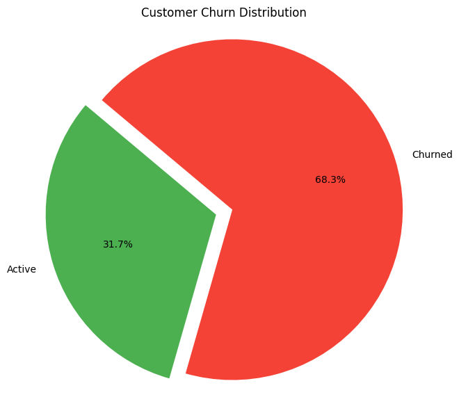
Out of 629,389 unique purchasing customers, 63.4% have churned, which means the number of churned customers is approximately 2 times greater than active customers.
To prevent further churn, especially within the 90-day window, we recommend regular retention initiatives, such as special events during payday or exclusive promotions (e.g., Black Market sales) at least once a month to recapture their attention.
Before launching campaigns, conducting behavioral analysis or customer surveys on churned users is essential to better understand their preferences, ensuring that the campaign is relevant, personalized, and impactful.
3. RFM
First of all, i need to make a measure of Recency, Frequency, and Monetary values of each customer. i choose maximum date of the data purchase became the comparation for the Recency value.
reference_date = df_purchase['purchase_date'].max()

rfm = df_purchase.groupby('customer_id').agg({
    'purchase_date': lambda x: (reference_date - x.max()).days,
    'transaction_id': 'nunique',
    'price': 'sum'
}).rename(columns={'purchase_date': 'Recency', 'transaction_id': 'Frequency', 'price': 'Monetary'})
After got the Recency, Frequency, and Monetary values. I divided the Recency, Frequency, and Monetary values into 4 categories.
rfm['R_score'] = pd.qcut(rfm['Recency'], 4, labels=[4,3,2,1]).astype(int)

try:
    rfm['F_score'] = pd.qcut(rfm['Frequency'].rank(method='dense'), 4, labels=[1,2,3,4]).astype(int)
except ValueError:
    rfm['F_score'] = pd.cut(rfm['Frequency'], bins=4, labels=[1,2,3,4]).astype(int)

try:
    rfm['M_score'] = pd.qcut(rfm['Monetary'].rank(method='dense'), 4, labels=[1,2,3,4]).astype(int)
except ValueError:
    rfm['M_score'] = pd.cut(rfm['Monetary'], bins=4, labels=[1,2,3,4]).astype(int)

rfm['RFM_Score'] = rfm['R_score'].astype(str) + rfm['F_score'].astype(str) + rfm['M_score'].astype(str)
The reason I applied pd.qcut directly on the Recency score is because Recency is a continuous variable with a wide range of values, making it suitable for quantile-based binning without additional processing.
On the other hand, Frequency and Monetary scores are discrete variables. Frequency often has a relatively small set of possible values, and Monetary values can be highly skewed and unevenly distributed.
Because of this, to effectively split Frequency and Monetary into 4 meaningful categories, I first applied ranking (rank()) to transform their discrete or skewed distributions into a more continuous-like scale. Then, I applied pd.qcut on these ranked values to get balanced quartile bins.
Then i need to make segmentation based on Recency, Frequency, and Monetary scores.
def segment_rfm(row):
    if row['RFM_Score'] == '444':
        return 'Champions'
    elif row['R_score'] >= 3 and row['F_score'] >= 3:
        return 'Loyal Customers'
    elif row['R_score'] >= 3 and row['M_score'] >= 3:
        return 'Big Spenders'
    elif row['R_score'] == 4:
        return 'Recent Customers'
    elif row['F_score'] >= 3:
        return 'Frequent Buyers'
    else:
        return 'At Risk'

rfm['Segment'] = rfm.apply(segment_rfm, axis=1)
And the result of the segmentation attached below
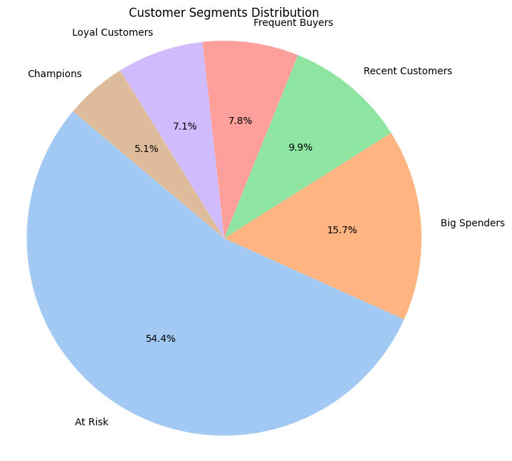
54% of our customers fall into the At Risk segment, meaning more than half of our customer base is at risk of churning or has significantly reduced engagement. This is a critical warning sign that immediate retention efforts are necessary to prevent revenue loss.
Recommendations:
Personalized engagement: Reach out with surveys or request feedback to make these customers feel valued and heard.
Targeted promotions: Offer incentives like discounts, vouchers, or free products to encourage reactivation.
Loyalty programs: Develop reward systems or communities to strengthen customer attachment and long-term loyalty.
For customers outside the At Risk segment:
Upselling and cross-selling: Promote new products with attractive offers such as buy-one-get-one or free samples.
Regular communication: Send relevant and engaging content tailored to their profile to maintain ongoing interest.
4. ARIMA
The first step before processing data using the ARIMA method is to check the ADF test statistic and its p-value.
This is important to determine whether the data is stationary or not. In my case, the data I am using consists of monthly clicks.
from statsmodels.tsa.arima.model import ARIMA
from statsmodels.tsa.stattools import adfuller

df_ads['date'] = pd.to_datetime(df_ads['date'])
daily_clicks = df_ads.groupby('date')['clicks'].sum().asfreq('D')

daily_clicks = daily_clicks.fillna(0)

result = adfuller(daily_clicks)
print('ADF Statistic:', result[0])
print('p-value:', result[1])
The results of the ADF test statistic and p-value are as follows:
ADF Statistic: -12.054420491695716
p-value: 2.553072882245295e-22
Since the p-value is less than 0.05, we can conclude that the data is already stationary. Therefore, no data transformation or differencing is needed.
Next, because no differencing or transformation is performed, the next step is to analyze the ACF and PACF plots to determine the appropriate orders of the Moving Average (MA) and Auto-Regressive (AR) components.
from statsmodels.graphics.tsaplots import plot_acf, plot_pacf
import matplotlib.pyplot as plt

fig, axes = plt.subplots(1, 2, figsize=(12, 5))

plot_acf(daily_clicks, ax=axes[0])
axes[0].set_title('ACF')

plot_pacf(daily_clicks, ax=axes[1])
axes[1].set_title('PACF')

plt.show()
The code produced the following ACF and PACF plots:
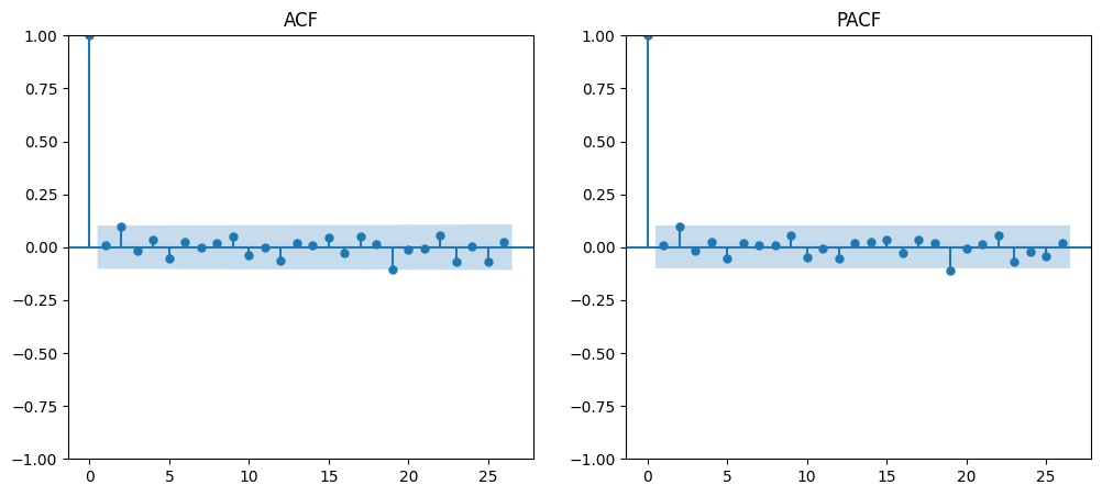
From the plots, it can be seen that both the ACF and PACF show a sharp decline after lag 0. Therefore, the possible ARIMA models could be ARIMA(0,0,0), ARIMA(1,0,0), ARIMA(0,0,1), or ARIMA(1,0,1).
Since several ARIMA models have been tested, the next step is to perform ARIMA analysis to determine the most suitable model.
This involves evaluating the models based on statistical metrics such as AIC, BIC, and residual diagnostics, in order to select the model that best fits the data.
ARIMA Model Comparison
| Metric | ARIMA(0,0,0) | ARIMA(1,0,0) | ARIMA(0,0,1) | ARIMA(1,0,1) |
|---|---|---|---|---|
| Dependent Variable | clicks | clicks | clicks | clicks |
| Observations | 366 | 366 | 366 | 366 |
| Log Likelihood | -2894.813 | -2894.794 | -2894.797 | -2894.340 |
| AIC | 5793.627 | 5795.589 | 5795.595 | 5796.680 |
| BIC | 5801.432 | 5807.297 | 5807.303 | 5812.290 |
| HQIC | 5796.729 | 5800.241 | 5800.247 | 5802.883 |
Coefficients
| Variable | ARIMA(0,0,0) | ARIMA(1,0,0) | ARIMA(0,0,1) | ARIMA(1,0,1) |
|---|---|---|---|---|
| const | 82,150 | 82,150 | 82,400 | 82,340 |
| ar.L1 | - | -0.1076 | - | 0.3605 |
| ma.L1 | - | - | -0.9976 | -1.0000 |
| sigma² | 14,220,000 | 14,680,000 | 9,616,000 | 9,245,000 |
Coefficient Significance (P>|z|)
| Variable | ARIMA(0,0,0) | ARIMA(1,0,0) | ARIMA(0,0,1) | ARIMA(1,0,1) |
|---|---|---|---|---|
| const | 0.000 | 0.000 | 0.000 | 0.000 |
| ar.L1 | - | 0.852 | - | 0.193 |
| ma.L1 | - | - | 0.876 | 0.241 |
| sigma² | 0.000 | 0.000 | 0.000 | 0.000 |
Residual Diagnostics
| Test | ARIMA(0,0,0) | ARIMA(1,0,0) | ARIMA(0,0,1) | ARIMA(1,0,1) |
|---|---|---|---|---|
| Ljung-Box (Q) | 0.04 | 0.00 | 0.00 | 0.32 |
| Prob(Q) (p-value) | 0.85 | 0.99 | 0.99 | 0.57 |
| Jarque-Bera (JB) | 13.22 | 13.22 | 13.22 | 13.78 |
| Prob(JB) (p-value) | 0.00 | 0.00 | 0.00 | 0.00 |
| Heteroskedasticity (H) | 0.92 | 0.92 | 0.92 | 0.93 |
| Prob(H) | 0.63 | 0.64 | 0.64 | 0.69 |
| Skewness | 0.46 | 0.46 | 0.46 | 0.47 |
| Kurtosis | 3.11 | 3.11 | 3.11 | 3.11 |
From the four models, ARIMA(0,0,0) is the best model based on having the lowest AIC and BIC values among all candidates. Although its log likelihood is slightly lower than other models, the difference is minimal and does not outweigh its advantage in AIC and BIC.
The drawback of this model is its relatively large sigma² value, which indicates greater variance in the residuals, potentially leading to wider confidence intervals in forecasts. However, given the primary objective of minimizing AIC and BIC for model selection, ARIMA(0,0,0) is still considered the superior choice among the models evaluated.
Based on the ARIMA modeling results, no significant trend component was detected in the dataset. This is likely due to the relatively short data period, consisting of only 12 monthly observations.
Forecast decided using ARIMA (0,0,0)
model = ARIMA(daily_clicks, order=(0, 0, 0))
model_fit = model.fit()

forecast = model_fit.forecast(steps=9)
The result of forecast by using Model ARIMA (0,0,0)
| Date | Predicted Mean |
|---|---|
| 2025-01-01 | 2693.601056 |
| 2025-01-02 | 2693.601056 |
| 2025-01-03 | 2693.601056 |
| 2025-01-04 | 2693.601056 |
| 2025-01-05 | 2693.601056 |
| 2025-01-06 | 2693.601056 |
| 2025-01-07 | 2693.601056 |
| 2025-01-08 | 2693.601056 |
| 2025-01-09 | 2693.601056 |
forecast_index = pd.date_range(start=daily_clicks.index[-1] + pd.Timedelta(days=1), periods=9, freq='D')

plt.figure(figsize=(12, 5))
plt.plot(daily_clicks.index, daily_clicks, label='Actual')
plt.plot(forecast_index, forecast, label='Forecast', marker='o', linestyle='--', color='orange')
plt.title('Daily Clicks Forecast')
plt.xlabel('Date')
plt.ylabel('Clicks')
plt.legend()
plt.grid(True)
plt.tight_layout()
plt.show()
The result of plot with actual data and predicted by using Model ARIMA (0,0,0)

For more accurate trend detection in time series analysis, it is generally recommended to use datasets with at least 24 or more observations to capture potential long-term trends or seasonal patterns.
Alternatively, employing other models such as SARIMA or Prophet would be more suitable for identifying trend and seasonality components, especially in datasets expected to have recurring patterns or long-term directional movements.
5. Behaviour Funnel
I have data for behaviour funnel, using impressions, clicks, leads, and transaction
Impressions: 18235179
Clicks: 985858 (CTR: 5.41%)
Leads: 985858 (Lead Conversion: 100.00%)
Purchases: 1132881 (Purchase Conversion: 114.91%)
and the funnel will show as this
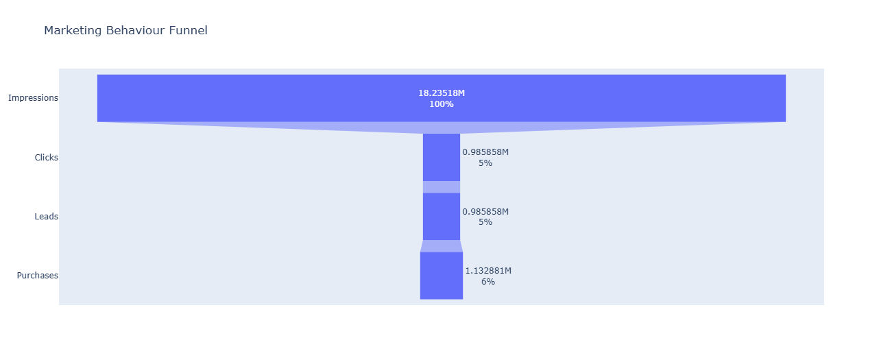
The significant gap between impressions and clicks indicates an opportunity for improvement. To increase engagement, we should create more interactive ads that truly resonate with the audience—ads that reflect their interests and follow current trends.
For example, if our product targets Gen Z, the ad content must align with trends popular among this group. Additionally, fine-tuning ad settings such as age, gender, and other demographics will help us reach the right customers more effectively.
By tailoring both the creative content and the targeting settings, we can increase click-through rates and ultimately generate more leads.